Lysario – by Panagiotis Chatzichrisafis
"ούτω γάρ ειδέναι το σύνθετον υπολαμβάνομεν, όταν ειδώμεν εκ τίνων και πόσων εστίν …"
Steven M. Kay: “Modern Spectral Estimation – Theory and Applications”,p. 61 exercise 3.7
Author: Panagiotis25 Apr
In [1, p. 61 exercise 3.7] we are asked to find the MLE of  and
and  .
for the conditions of Problem [1, p. 60 exercise 3.4] (see also [2, solution of exercise 3.4]).
We are asked if the MLE of the parameters are asymptotically unbiased , efficient and Gaussianly distributed.
.
for the conditions of Problem [1, p. 60 exercise 3.4] (see also [2, solution of exercise 3.4]).
We are asked if the MLE of the parameters are asymptotically unbiased , efficient and Gaussianly distributed.
Solution:
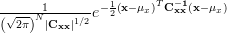
The p.d.f of the observations![\mathbf{x}=\left[ \begin{array}{cccc} x_{1} & x_{2} & ... & x_{ n} \end{array} \right]](https://lysario.de/wp-content/cache/tex_1b1152d0095c0b64c283a57f268936c3.png) is given by
is given by
With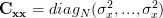 and
and 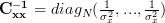 . Thus the determinant is given by
  . Furthermore we can simplify

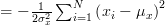 For a given measurement
  we obtain the likelihood function:
Obviously the previous equation is positive and thus the estimator of the mean which will maximize the probability of the observation
  will provide a local maximum at the points where the derivative in respect to
  will be zero. Because the function is positive we can also use the natural logarithm of the likelihood function (the log-likelihood function) in order to obtain the maximum likelihood of
  . This was already derived in
[3, relation (3)]:
. This was already derived in
[3, relation (3)]:
From the previous relation we derive the maximum likelihood estimator of:
With the same reasoning we may obtain the maximum likelihood estimator of the variance :
:
Again solving for will give us the maximum likelihood estimator of the variance of the random process:
The mean of the maximum likelihood estimator of the variance can be easily obtained using [4, relation (8)] and noting that the maximum likelihood estimator of the variance is times the variance estimator that was used in [1, p. 61 exercise 3.6] (see also [4, solution of exercise 3.6]):
The variance of the maximum likelihood estimator of the variance can be obtained by analogy to [4] by noting that
From the previous relation we can obtain the variance of the maximum likelihood variance estimator by:
By using the results from this exercise and [2], [4] we can summarize the properties of the MLE estimators in the following table:
From the previous table it is evident that for large the mean values of the estimators match the true mean values. The same is true for the variances that asymptotically tend to zero – the same limit the CR – bound attains for
  . The MLE estimator of the mean is Gaussianly distributed even for small , while by the central limit theorem [5, p. 622] the MLE estimator of the variance
  () is also asymptotically distributed Gaussianly. So the answer to the question if the parameters are asymptotically unbiased, efficient and Gaussianly distributed is yes. QED.
[1] Steven M. Kay: “Modern Spectral Estimation – Theory and Applications”, Prentice Hall, ISBN: 0-13-598582-X.
[2] Chatzichrisafis: “Solution of exercise 3.4 from Kay’s Modern Spectral Estimation - Theory and Applications”.
[3] Chatzichrisafis: “Solution of exercise 3.5 from Kay’s Modern Spectral Estimation - Theory and Applications”.
[4] Chatzichrisafis: “Solution of exercise 3.6 from Kay’s Modern Spectral Estimation - Theory and Applications”.
[5] Granino A. Korn and Theresa M. Korn: “Mathematical Handbook for Scientists and Engineers”, Dover, ISBN: 978-0-486-41147-7.
and .
for the conditions of Problem [1, p. 60 exercise 3.4] (see also [2, solution of exercise 3.4]).
We are asked if the MLE of the parameters are asymptotically unbiased , efficient and Gaussianly distributed. Solution:
The p.d.f of the observations
is given by
 |  |  |
With
and . Thus the determinant is given by . Furthermore we can simplify
For a given measurement we obtain the likelihood function:
 | (1) | ||
Obviously the previous equation is positive and thus the estimator of the mean
which will maximize the probability of the observation will provide a local maximum at the points where the derivative in respect to will be zero. Because the function is positive we can also use the natural logarithm of the likelihood function (the log-likelihood function) in order to obtain the maximum likelihood of . This was already derived in
[3, relation (3)]:
 | |  | |
![\frac{\partial \left(-\frac{N}{2}\ln(2\pi \sigma^{2}_x)-\frac{1}{2}\sum\limits_{i=0}^{N-1}\left(\frac{x^{\prime}[i]-\hat{\mu}_x}{\sigma_x}\right)^2\right)}{\partial \hat{\mu}_{x}}](https://lysario.de/wp-content/cache/tex_393cc6672687c8e103f89da2bac7061b.png) | | | |
![\frac{1}{\sigma_{x}^{2}}\sum\limits_{i=0}^{N-1}\left(x^{\prime}[i]-\hat{\mu}_x\right)](https://lysario.de/wp-content/cache/tex_af01b61bd038311f28e62116562b609f.png) | |  | |
 | | ![\sum\limits_{i=0}^{N-1}\left(x^{\prime}[i]\right)](https://lysario.de/wp-content/cache/tex_8b90a25227a02b12efbe3ceb59901494.png) |
From the previous relation we derive the maximum likelihood estimator of
:
 | | ![\frac{\sum\limits_{i=0}^{N-1}\left(x^{\prime}[i]\right)}{N}](https://lysario.de/wp-content/cache/tex_ede2cd3b1ff0a5370cc7dfe4765a38cf.png) | (2) |
With the same reasoning we may obtain the maximum likelihood estimator of the variance
:
 | | | |
![\frac{\partial \left(-\frac{N}{2}\ln(2\pi \hat{\sigma}^{2}_x)-\frac{1}{2}\sum\limits_{i=0}^{N-1}\left(\frac{x^{\prime}[i]-\hat{\mu}_x}{\hat{\sigma}_x}\right)^2\right)}{\partial \hat{\sigma}^{2}_{x}}](https://lysario.de/wp-content/cache/tex_bc621add9e5d8d08838d0d8a53d35230.png) | | | |
![-\frac{N}{2\hat{\sigma}_{x}^{2}}+\frac{1}{\hat{\sigma}^{4}}\sum\limits_{i=0}^{N-1}\left(x^{\prime}[i]-\hat{\mu}_{x}\right)^{2}](https://lysario.de/wp-content/cache/tex_33ab2eb97907df96f8105cb964569e24.png) | | |
Again solving for
will give us the maximum likelihood estimator of the variance of the random process:
| | ![\frac{1}{N}\sum\limits_{i=0}^{N-1}\left(x^{\prime}[i]-\hat{\mu}_{x}\right)^{2}](https://lysario.de/wp-content/cache/tex_92b017730c1caa9dd302d4b10c92f1b3.png) | (3) |
The mean of the maximum likelihood estimator of the variance can be easily obtained using [4, relation (8)] and noting that the maximum likelihood estimator of the variance is
times the variance estimator that was used in [1, p. 61 exercise 3.6] (see also [4, solution of exercise 3.6]):
 | |  | (4) |
The variance of the maximum likelihood estimator of the variance can be obtained by analogy to [4] by noting that
 | |||
From the previous relation we can obtain the variance of the maximum likelihood variance estimator by:
 | |  | |
|  | ||
|  | ||
|  | (5) |
By using the results from this exercise and [2], [4] we can summarize the properties of the MLE estimators
in the following table:
![\begin{array}{lcc}
MLE & \hat{\mu}_x = \frac{\sum_{i=0}^{N-1}\left(x^{\prime}[i]\right)}{N} & \hat{\sigma}_{x}^{2}=\frac{1}{N}\sum_{i=0}^{N-1}\left(x^{\prime}[i]-\hat{\mu}_{x}\right)^{2} \\
\hline
mean & \mu_{x} & \frac{N-1}{N} \sigma^{2}_{x} \\
\hline
variance &\frac{\sigma^{2}_{x}}{N} & \frac{2 \sigma_{x}^{4}(N-1)}{N^{2}} \\
\hline
CR-bound & \frac{\sigma^{2}_{x}}{N} & \frac{2\sigma_{x}^{4}}{N} \\
\hline
distribution & \sim N(\mu_{x},\sigma^{2}_{x}) & \sim \chi^{2}_{N-1}
\end{array}](https://lysario.de/wp-content/cache/tex_9f791e8f343583312466711212b006d2.png) | |||
From the previous table it is evident that for large
the mean values of the estimators match the true mean values. The same is true for the variances that asymptotically tend to zero – the same limit the CR – bound attains for . The MLE estimator of the mean is Gaussianly distributed even for small , while by the central limit theorem [5, p. 622] the MLE estimator of the variance () is also asymptotically distributed Gaussianly. So the answer to the question if the parameters are asymptotically unbiased, efficient and Gaussianly distributed is yes. QED.
[1] Steven M. Kay: “Modern Spectral Estimation – Theory and Applications”, Prentice Hall, ISBN: 0-13-598582-X.
[2] Chatzichrisafis: “Solution of exercise 3.4 from Kay’s Modern Spectral Estimation - Theory and Applications”.
[3] Chatzichrisafis: “Solution of exercise 3.5 from Kay’s Modern Spectral Estimation - Theory and Applications”.
[4] Chatzichrisafis: “Solution of exercise 3.6 from Kay’s Modern Spectral Estimation - Theory and Applications”.
[5] Granino A. Korn and Theresa M. Korn: “Mathematical Handbook for Scientists and Engineers”, Dover, ISBN: 978-0-486-41147-7.
Leave a reply