Lysario – by Panagiotis Chatzichrisafis
"ούτω γάρ ειδέναι το σύνθετον υπολαμβάνομεν, όταν ειδώμεν εκ τίνων και πόσων εστίν …"
Steven M. Kay: “Modern Spectral Estimation – Theory and Applications”,p. 61 exercise 3.6
Author: Panagiotis19 Apr
In [1, p. 61 exercise 3.6] we are asked to assume that the variance is to be estimated as well as the mean for the conditions of [1, p. 60 exercise 3.4] (see also [2, solution of exercise 3.4]) . We are asked to prove for the vector parameter ![\mathbf{\theta}=\left[\mu_x \; \sigma^2_x\right]^T](https://lysario.de/wp-content/cache/tex_b1d973967798bb8525bff936468f9211.png) , that the Fisher information matrix is
, that the Fisher information matrix is
Furthermore we are asked to find the CR bound and to determine if the sample mean is efficient.
If additionaly the variance is to be estimated as
is efficient.
If additionaly the variance is to be estimated as
then we are asked to determine if this estimator is unbiased and efficient. Hint: We are instructed to use the result that
Solution: We have already obtained the joint pdf of the
  independent samples with normal distribution
  and the natural logarithm of the joint pdf is given by from [3, relation (3) ]:
From this relation we can find the gradient in respect to the vector parameter:
Thus Fisher’s information matrix is given by [1, p. 47, (3.22) ]:
Considering that the samples![x[i] \;, i=0,..,N](https://lysario.de/wp-content/cache/tex_47214f3be4a9f9fabf23ed367fe4f59e.png) are independent we obtain the individual elements of the matrix
are independent we obtain the individual elements of the matrix  are given by:
We note that![h(x[i])=\left(\frac{x[i]-\mu_x}{\sigma^{2}_x} \right)^{3}](https://lysario.de/wp-content/cache/tex_c6732a1b8dbe5a4501adfb197b65a1f3.png) is an odd function about
is an odd function about  (that is
  ) while the gaussian distribution is an even function about
  . Thus the mean of this function -the integral which is symmetric about and extends from
  to
to  will be equal to zero. This fact can be shown by the following approach:
Let![u=\left(x[i]-\mu_{x}\right)](https://lysario.de/wp-content/cache/tex_ba7b6d07b92b8d66bab0265749653ea1.png) in the last formula
in the last formula
If we set in the second integral, we obtain the following formulas:
Using [2] in conjunction with [3] we obtain
Finally it remains to obtain the value for :
:
We note that![v_{i}=\frac{x[i]-\mu_x}{\sigma_x}](https://lysario.de/wp-content/cache/tex_ffdcad199afcc8629b93660aeb6dafe4.png) in (5) is a normalized random gaussian variable and that the squared sum of such variables
in (5) is a normalized random gaussian variable and that the squared sum of such variables
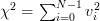 has a chi-square distribution [4, p. 682] with N degrees of freedom with mean
  and variance equal to
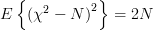 . Thus
From (1), (4) and (6) we obtain finally that Fisher’s information matrix is equal to:
We have shown in [2, solution of exercise 3.4] that the mean and the variance [2, solution of exercise 3.4, relation (5) ] of the estimator are given by:
The mean and the variance of the estimator are given by (always considering the independence of the random variables
 ![x[n], x[k]](https://lysario.de/wp-content/cache/tex_2b0db6c4a3986293f7b951e7c4a9de00.png) for
for  ):
):
From the previous relation we obtain finally:
Considering that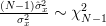 we can also obtain the variance of the estimator
  :
:
Because the Cramer Rao bound for the estimator is given by the inverse of the diagonal element of Fisher’s information matrix (6) we obtain using (9) :
thus the estimator is unbiased because of (8) but not efficient because it doesn’t attain the Cramer – Rao bound given by (10).
QED.
[1] Steven M. Kay: “Modern Spectral Estimation – Theory and Applications”, Prentice Hall, ISBN: 0-13-598582-X.
[2] Chatzichrisafis: “Solution of exercise 3.4 from Kay’s Modern Spectral Estimation - Theory and Applications”.
[3] Chatzichrisafis: “Solution of exercise 3.5 from Kay’s Modern Spectral Estimation - Theory and Applications”.
[4] Granino A. Korn and Theresa M. Korn: “Mathematical Handbook for Scientists and Engineers”, Dover, ISBN: 978-0-486-41147-7.
, that the Fisher information matrix is
![\mathbf{I}_{\theta}=\left[\begin{array}{cc} \frac{N}{\sigma^2_x} & 0 \\ 0 & \frac{N}{2\sigma^4_x} \end{array}\right]](https://lysario.de/wp-content/cache/tex_42789b24f24a6a32db03314ccac291c8.png) | |||
Furthermore we are asked to find the CR bound and to determine if the sample mean
is efficient.
If additionaly the variance is to be estimated as
![\hat{\sigma}^2_x=\frac{1}{N-1}\sum\limits_{n=0}^{N-1}(x[n]-\hat{\mu}_x)^2](https://lysario.de/wp-content/cache/tex_13d6ef5f9b8f0b1d9832efd9b58af88b.png) | |||
then we are asked to determine if this estimator is unbiased and efficient. Hint: We are instructed to use the result that
| |||
Solution: We have already obtained the joint pdf
of the independent samples with normal distribution and the natural logarithm of the joint pdf is given by from [3, relation (3) ]:
 |  | ![-\ln(\sqrt{2\pi}\sigma_x)N-\frac{1}{2}\sum\limits_{i=0}^{N-1}\left(\frac{x[i]-\mu_x}{\sigma_x}\right)^2](https://lysario.de/wp-content/cache/tex_d70aee1bec5c1013d3e79f140db20654.png) | |
| ![-\frac{N}{2}\ln(2\pi \sigma^{2}_x)-\frac{1}{2}\sum\limits_{i=0}^{N-1}\left(\frac{x[i]-\mu_x}{\sigma_x}\right)^2](https://lysario.de/wp-content/cache/tex_b0debdaa5cd11556e9c4db5a4490619b.png) |
From this relation we can find the gradient in respect to the vector parameter:
 | | ![\left[ \begin{array}{cc} \frac{\partial \ln(f(\mathbf{x};\theta))}{\partial \mu_{x}} & \frac{\partial \ln(f(\mathbf{x};\theta))}{\partial \sigma^{2}_{x}} \end{array} \right]^{T}](https://lysario.de/wp-content/cache/tex_8f8126a7cecf6f0790fec3dc60b117dc.png) | |
| ![\left[ \begin{array}{cc} \sum_{i=0}^{N-1}\left(\frac{x[i]-\mu_x}{\sigma^{2}_x}\right) & -\frac{N}{2\sigma_{x}^{2}}+\frac{1}{2} \sum_{i=0}^{N-1}\frac{\left(x[i]-\mu_x\right)^2}{\sigma^{4}_x}\end{array} \right]^{T}](https://lysario.de/wp-content/cache/tex_316fe977824c4e41b259a44eb32121e0.png) |
Thus Fisher’s information matrix is given by [1, p. 47, (3.22) ]:
 | |  |
Considering that the samples
are independent we obtain the individual elements of the matrix are given by:
 | | ![E\left\{ \left(\sum\limits_{i=0}^{N-1}\left(\frac{x[i]-\mu_x}{\sigma^{2}_x}\right) \right)^{2} \right\}](https://lysario.de/wp-content/cache/tex_792f46c5e2010423fd7d5530c704ebce.png) | |
| ![E\left\{ \sum\limits_{i=0}^{N-1}\frac{\left(x[i]-\mu_x\right)^{2}}{\sigma^{4}_x} +\sum\limits_{i=0}^{N-1}\sum\limits_{j=0,j\neq i}^{N-1}\frac{\left(x[i]-\mu_x\right)\left(x[j]-\mu_x\right)}{\sigma^{4}_x} \right\}](https://lysario.de/wp-content/cache/tex_753e53f6b6a2aafe935f391d3f0e3fab.png) | ||
| ![\sum\limits_{i=0}^{N-1}\frac{E\left\{ \left(x[i]-\mu_x\right)^{2}\right\}}{\sigma^{4}_x}](https://lysario.de/wp-content/cache/tex_8bf310ccf6cecd51efd069b42ed7d317.png) | ||
 | ![+\sum\limits_{i=0}^{N-1}\sum\limits_{j=0,j\neq i}^{N-1}\frac{E\left\{\left(x[i]-\mu_x\right)\right\}E\left\{\left(x[j]-\mu_x\right)\right\}}{\sigma^{4}_x}](https://lysario.de/wp-content/cache/tex_928ebf2a7a124a71aec67749671b167d.png) | ||
|  | ||
|  | (1) | |
 | | ![E\left\{ \left(\sum\limits_{i=0}^{N-1}\left(\frac{x[i]-\mu_x}{\sigma^{2}_x}\right) \right) \left(-\frac{N}{2\sigma_{x}^{2}}+\frac{1}{2} \sum\limits_{i=0}^{N-1}\frac{\left(x[i]-\mu_x\right)^2}{\sigma^{4}_x}\right) \right\}](https://lysario.de/wp-content/cache/tex_c04b3f411453cd48319328d58820ebe6.png) | |
| ![E\left\{ -\frac{N}{2 \sigma_{x}^{2} } \sum\limits_{i=0}^{N-1} \left(\frac{x[i]-\mu_x}{\sigma^{2}_x}\right)\right\}](https://lysario.de/wp-content/cache/tex_73a6d5b8ec75fc97dda66f145453710b.png) | ||
| ![+E\left\{ \left(\sum\limits_{i=0}^{N-1}\frac{x[i]-\mu_x}{\sigma^{2}_x} \right) \left(\frac{1}{2}\sum\limits_{i=0}^{N-1}\frac{\left( x[i]-\mu_x \right)^2}{\sigma^{4}_x}\right) \right\}](https://lysario.de/wp-content/cache/tex_aba4104a454ffb06677a3ae02775d202.png) | ||
| ![-\frac{N}{2 \sigma_{x}^{2} } \sum\limits_{i=0}^{N-1} \left(\frac{E\left\{x[i]\right\}-\mu_x}{\sigma^{2}_x}\right)
+\frac{1}{2}E\left\{ \sum\limits_{i=0}^{N-1}\left(\frac{x[i]-\mu_x}{\sigma^{2}_x} \right)^{3}\right\}](https://lysario.de/wp-content/cache/tex_010392e342611bc4911507b6a786915d.png) | ||
| ![+ \frac{1}{2}E\left\{\sum\limits_{i=0}^{N-1} \sum\limits_{j=0,j\neq i}^{N-1}\frac{\left(x[j]-\mu_x\right)\left( x[i]-\mu_x \right)^2}{\sigma^{6}_x} \right\}](https://lysario.de/wp-content/cache/tex_e3f4c83432f37c3a544bafd8844c5472.png) | ||
| ![0+\frac{1}{2} E\left\{ \sum\limits_{i=0}^{N-1}\left(\frac{x[i]-\mu_x}{\sigma^{2}_x} \right)^{3}\right\}](https://lysario.de/wp-content/cache/tex_78286af501c19fc5483328ddaec0be5b.png) | ||
| ![+\frac{1}{2}\sum\limits_{i=0}^{N-1} \sum\limits_{j=0,j\neq i}^{N-1}\frac{ E\left\{\left(x[j]-\mu_x\right)\left( x[i]-\mu_x \right)^2\right\}}{\sigma^{6}_x}](https://lysario.de/wp-content/cache/tex_9d8ab121240ac809606624347a76410c.png) | ||
| ![\frac{1}{2}E\left\{ \sum\limits_{i=0}^{N-1}\left(\frac{x[i]-\mu_x}{\sigma^{2}_x} \right)^{3}\right\}](https://lysario.de/wp-content/cache/tex_7ebdfee13e758847e5f688c756467083.png) | ||
| ![+\frac{1}{2}\sum\limits_{i=0}^{N-1} \sum\limits_{j=0,j\neq i}^{N-1}\frac{ E\left\{\left(x[j]-\mu_x\right)\right\}E\left\{\left( x[i]-\mu_x \right)^2\right\}}{\sigma^{6}_x}](https://lysario.de/wp-content/cache/tex_12f77a724849dcd55fabe1b005221eed.png) | ||
| ![\frac{1}{2} E\left\{ \sum\limits_{i=0}^{N-1}\left(\frac{x[i]-\mu_x}{\sigma^{2}_x} \right)^{3}\right\} +0](https://lysario.de/wp-content/cache/tex_6ef454ab2a25b36d61fc59e8a5cd4465.png) | ||
| ![\frac{1}{2} \sum\limits_{i=0}^{N-1}E\left\{\left(\frac{x[i]-\mu_x}{\sigma^{2}_x} \right)^{3} \right\}](https://lysario.de/wp-content/cache/tex_bed7fc9813146d9c54133fce464e5383.png) | (2) |
We note that
is an odd function about (that is ) while the gaussian distribution is an even function about . Thus the mean of this function -the integral which is symmetric about and extends from to will be equal to zero. This fact can be shown by the following approach:
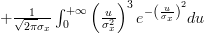
![E\left\{\left(\frac{x[i]-\mu_x}{\sigma^{2}_x} \right)^{3} \right\}](https://lysario.de/wp-content/cache/tex_afca19da303893e83b6fcffb7182e25e.png) | | ![\frac{1}{\sqrt{2\pi}\sigma_{x}}\int_{-\infty}^{+\infty}\left(\frac{x[i]-\mu_x}{\sigma^{2}_x} \right)^{3}e^{-\left(\frac{x[i]-\mu_{x}}{\sigma_{x}}\right)^{2}} dx](https://lysario.de/wp-content/cache/tex_3c9f7e91efb09b74d9bdd80c47965fac.png) | |
| ![\frac{1}{\sqrt{2\pi}\sigma_{x}}\int_{-\infty}^{\mu_{x}}\left(\frac{x[i]-\mu_x}{\sigma^{2}_x} \right)^{3}e^{-\left(\frac{x[i]-\mu_{x}}{\sigma_{x}}\right)^{2}} dx](https://lysario.de/wp-content/cache/tex_4e9064648161579be317450b6cddf0ae.png) | ||
| ![+\frac{1}{\sqrt{2\pi}\sigma_{x}}\int_{\mu_{x}}^{+\infty}\left(\frac{x[i]-\mu_x}{\sigma^{2}_x} \right)^{3}e^{-\left(\frac{x[i]-\mu_{x}}{\sigma_{x}}\right)^{2}} dx](https://lysario.de/wp-content/cache/tex_6263ae551b2578a05f7f5b86c0a404af.png) |
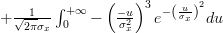
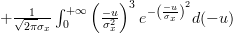
Let
in the last formula
|  |  | |
|  | ||
| | ||
|  | ||
| | ||
|  |
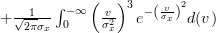
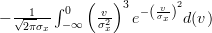
If we set
in the second integral, we obtain the following formulas:
| |  | |
|  | ||
|  | ||
|  | ||
| |  | (3) |
Using [2] in conjunction with [3] we obtain
 | (4) | ||
Finally it remains to obtain the value for
:
| | ![E\left\{\left( -\frac{N}{2\sigma_{x}^{2}}+\frac{1}{2} \sum\limits_{i=0}^{N-1}\frac{\left(x[i]-\mu_x\right)^2}{\sigma^{4}_x}\right)^{2}\right\}](https://lysario.de/wp-content/cache/tex_ebff0c112204a26381e1b6d2e195131d.png) | |
| ![\frac{1}{4\sigma_{x}^{4}} E\left\{\left( \sum\limits_{i=0}^{N-1}\left(\frac{x[i]-\mu_x}{\sigma_x}\right)^{2} -N\right)^{2}\right\}](https://lysario.de/wp-content/cache/tex_1407c36863a9d98363e7b66da305ee07.png) | (5) |
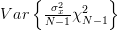
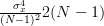
We note that
in (5) is a normalized random gaussian variable and that the squared sum of such variables
has a chi-square distribution [4, p. 682] with N degrees of freedom with mean and variance equal to
. Thus
 | (6) | ||
From (1), (4) and (6) we obtain finally that Fisher’s information matrix is equal to:
![\mathbf{I}_{\theta}=\left[ \begin{array}{cc} \frac{N}{\sigma_{x}^{2}} & 0 \\ 0 &\frac{N}{2\sigma_{x}^{4}} \end{array} \right].](https://lysario.de/wp-content/cache/tex_3b0698479493ccbebcb94f2b171905d4.png) | (7) | ||
We have shown in [2, solution of exercise 3.4] that the mean and the variance [2, solution of exercise 3.4, relation (5) ] of the estimator
are given by:
 | | | |
 | |  |
The mean and the variance of the estimator
are given by (always considering the independence of the random variables for ):
 | | ![\frac{1}{N-1}\sum\limits_{n=0}^{N-1}E\left\{(x[n]-\hat{\mu}_{x})^{2}\right\}](https://lysario.de/wp-content/cache/tex_cb3bcfe8a78cbcfe97e2e5bea783b5f6.png) | |
| ![\frac{1}{N-1}\sum\limits_{n=0}^{N-1}E\left\{((x[n]-\mu_{x})- (\hat{\mu}_{x}-\mu_{x}))^{2}\right\}](https://lysario.de/wp-content/cache/tex_231dd0454e424691213f11b75cbc92ce.png) | ||
| ![\frac{1}{N-1}\sum\limits_{n=0}^{N-1}E\left\{(x[n]-\mu_{x})^{2}\right\}+\frac{1}{N-1}\sum\limits_{n=0}^{N-1} E\left\{(\hat{\mu}_{x}-\mu_{x})^{2}\right\}](https://lysario.de/wp-content/cache/tex_3d00a79760b79a0e3848b68664988764.png) | ||
| ![- \frac{2}{N-1}\sum\limits_{n=0}^{N-1}E\left\{(x[n]-\mu_{x})(\hat{\mu}_{x}-\mu_{x})\right\}](https://lysario.de/wp-content/cache/tex_d8b2279930f39c7fc227f711592f0d18.png) | ||
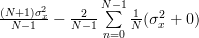
| ![\frac{N\sigma^{2}_{x}}{N-1} + \frac{\sigma^{2}_{x}}{N-1} - \frac{2}{N-1}\sum\limits_{n=0}^{N-1}E\left\{(x[n]-\mu_{x})(\hat{\mu}_{x}-\mu_{x})\right\}](https://lysario.de/wp-content/cache/tex_471dd6e5191e8180c8363b4f2ca415cc.png) | ||
| ![\frac{(N+1)\sigma^{2}_{x}}{N-1} - \frac{2}{N-1}\sum\limits_{n=0}^{N-1}E\left\{(x[n]-\mu_{x})(\hat{\mu}_{x}-\mu_{x})\right\}](https://lysario.de/wp-content/cache/tex_b010f17a02ef30803066e9744eff0902.png) | ||
| ![\frac{(N+1)\sigma^{2}_{x}}{N-1} - \frac{2}{N-1}\sum\limits_{n=0}^{N-1}E\left\{(x[n]-\mu_{x})(\frac{1}{N}\sum\limits_{i=0}^{N-1}x[i]-\mu_{x})\right\}](https://lysario.de/wp-content/cache/tex_799df226eef47a5c70ad69bf0a168ee4.png) | ||
| ![\frac{(N+1)\sigma^{2}_{x}}{N-1} - \frac{2}{N-1}\sum\limits_{n=0}^{N-1}E\left\{\frac{1}{N}(x[n]-\mu_{x})(\sum\limits_{i=0}^{N-1}(x[i]-\mu_{x}))\right\}](https://lysario.de/wp-content/cache/tex_c74f3bbf988a63c99ee0571016b2d8b7.png) | ||
|  | ||
| ![\frac{2}{N-1}\sum\limits_{n=0}^{N-1}\frac{1}{N}\Bigg( E\left\{(x[n]-\mu_{x})^{2}\right\}](https://lysario.de/wp-content/cache/tex_22c74ad89e814b2d8938483b6629a349.png) | ||
| ![\left. +\sum\limits_{i=0,i\neq n}^{N-1}E\left\{(x[n]-\mu_{x})(x[i]-\mu_{x})\right\} \right)](https://lysario.de/wp-content/cache/tex_f09a7fbef01d723cdd397005eb47e54d.png) | ||
| | ||
| 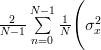 | ||
| ![+\sum\limits_{i=0,i\neq n}^{N-1}E\left\{(x[n]-\mu_{x})\right\}E\left\{(x[i]-\mu_{x})\right\} \Bigg)](https://lysario.de/wp-content/cache/tex_76d0bb291df21da89c9f62716bdb789e.png) | ||
|  | ||
|  |
From the previous relation we obtain finally:
| |  | (8) |
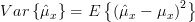
Considering that
we can also obtain the variance of the estimator :
 | |  | |
| 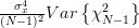 | ||
|  | ||
|  | (9) |
Because the Cramer Rao bound for the estimator
is given by the inverse of the diagonal element of Fisher’s information matrix (6) we obtain using (9) :
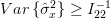 | |||
 | (10) | ||
thus the estimator
is unbiased because of (8) but not efficient because it doesn’t attain the Cramer – Rao bound given by (10).
QED.
[1] Steven M. Kay: “Modern Spectral Estimation – Theory and Applications”, Prentice Hall, ISBN: 0-13-598582-X.
[2] Chatzichrisafis: “Solution of exercise 3.4 from Kay’s Modern Spectral Estimation - Theory and Applications”.
[3] Chatzichrisafis: “Solution of exercise 3.5 from Kay’s Modern Spectral Estimation - Theory and Applications”.
[4] Granino A. Korn and Theresa M. Korn: “Mathematical Handbook for Scientists and Engineers”, Dover, ISBN: 978-0-486-41147-7.
One Response for "Steven M. Kay: “Modern Spectral Estimation – Theory and Applications”,p. 61 exercise 3.6"
[...] The mean of the maximum likelihood estimator of the variance can be easily obtained using [4, relation (8)] and noting that the maximum likelihood estimator of the variance is times the variance estimator [...]
Leave a reply