Lysario – by Panagiotis Chatzichrisafis
"ούτω γάρ ειδέναι το σύνθετον υπολαμβάνομεν, όταν ειδώμεν εκ τίνων και πόσων εστίν …"
Steven M. Kay: “Modern Spectral Estimation – Theory and Applications”,p. 60 exercise 3.2
Author: Panagiotis8 Nov
In [1, p. 60 exercise 3.2] we are asked to proof by using the method of characteristic functions that the sum of squares of N independent and identically distributed N(0,1) random variables has a  distribution.
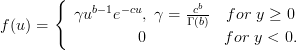
Solution: The distribution is by definition [2, p.302] the distribution of the sum of squares of N independent and identically distributed random variables and even [1, p. 43] doesn’t seem to give a different definition. By using this definition the solution of this exercise would be indeed really short. In the solution provided in the following text we will assume that the distribution is defined by [1, p.43, (3.7)], and we will show that the distribution can be derived also from the sum of N independent and identically distributed N(0,1) random variables by using characteristic functions.
First let us reproduce the probability density function of a variable
distribution is by definition [2, p.302] the distribution of the sum of squares of N independent and identically distributed random variables and even [1, p. 43] doesn’t seem to give a different definition. By using this definition the solution of this exercise would be indeed really short. In the solution provided in the following text we will assume that the distribution is defined by [1, p.43, (3.7)], and we will show that the distribution can be derived also from the sum of N independent and identically distributed N(0,1) random variables by using characteristic functions.
First let us reproduce the probability density function of a variable  that is distributed according to a distribution from [1, p.43, (3.7)]:
We note the close relation to the pdf of a random variable with gamma distribution [3, p.79, (4.38)]:
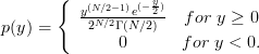
which is equal to the distribution for
  and
and  .
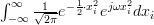
The characteristic function of a distribution with probability density function (pdf)
.
The characteristic function of a distribution with probability density function (pdf)  is given by [3] :
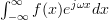
and can be derived from the moment generating function .
.
The moment generating function of the distribution is given by [3, p.117, (5.71)]: .
And by replacing with
with  we obtain from (2) the characteristic function of the pdf of the chi square distribution:
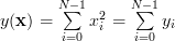
Now let us proceed to obtain the characteristic function of the random variable which we define to be that random variable that is obtained by the sum of squares of  independent and identically distributed N(0,1) random variables by using gaussian distributons. The variable is given by:
with![\mathbf{x} = \left[ \begin{array}{ccc}x_{0} &,..., & x_{N-1}\end{array} \right]^{T}](https://lysario.de/wp-content/cache/tex_0f7c6a342e20d6e512dcafa8275cb4d2.png) .
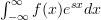
In order to compute the characteristic function of
.
In order to compute the characteristic function of  we will need the following theorem from [3, (5.32), p. 106]:
The characteristic function of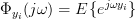 can thus be computed by (5).
The integral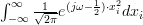 was evaluated using the integral tables of [4, p. 992]. We note that the joint probability density function
  of
of  is given by the product of the individual pdf’s of the normal distributed random variables
  , with
 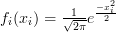 because the random variables are independent:
Thus the characteristic function of is given by [3, p. 158]:
which by using (6) is equal to:
By comparing the equation (3) with (8) we see that the same characteristic function is obtained by either using the probability density function as given by (1) or by computing the characteristic function using the squared sum of gaussian distributed random variables in conjunction with theorem (5). By virtue of the uniqueness theorem of Fourier transform pairs – the characteristic functions of a pdf is also a Fourier transform – we obtain the result that the probability density function of the squared sum of gaussian distributed random variables is equal to (1).
QED.
gaussian distributed random variables in conjunction with theorem (5). By virtue of the uniqueness theorem of Fourier transform pairs – the characteristic functions of a pdf is also a Fourier transform – we obtain the result that the probability density function of the squared sum of gaussian distributed random variables is equal to (1).
QED.
[1] Steven M. Kay: “Modern Spectral Estimation – Theory and Applications”, Prentice Hall, ISBN: 0-13-598582-X.
[2] Fahrmeir and Künstler and Pigeot and Tutz: “Statistik”, Springer.
[3] Papoulis, Athanasios: “Probability, Random Variables, and Stochastic Processes”, McGraw-Hill.
[4] Bronstein and Semdjajew and Musiol and Muehlig: “Taschenbuch der Mathematik”, Verlag Harri Deutsch Thun und Frankfurt am Main, ISBN: 3-8171-2003-6.
distribution.
Solution: The
distribution is by definition [2, p.302] the distribution of the sum of squares of N independent and identically distributed random variables and even [1, p. 43] doesn’t seem to give a different definition. By using this definition the solution of this exercise would be indeed really short. In the solution provided in the following text we will assume that the distribution is defined by [1, p.43, (3.7)], and we will show that the distribution can be derived also from the sum of N independent and identically distributed N(0,1) random variables by using characteristic functions.
First let us reproduce the probability density function of a variable that is distributed according to a distribution from [1, p.43, (3.7)]:
 | (1) | ||
We note the close relation to the pdf of a random variable
with gamma distribution [3, p.79, (4.38)]:
 | |||
which is equal to the
distribution for and .
The characteristic function of a distribution with probability density function (pdf) is given by [3] :
 |  |  | |
|  |
and can be derived from the moment generating function
.
| |  | |
|  |
The moment generating function of the
distribution is given by [3, p.117, (5.71)]: .
 | (2) | ||
And by replacing
with we obtain from (2) the characteristic function of the pdf of the chi square distribution:
 | (3) | ||
Now let us proceed to obtain the characteristic function of the random variable
which we define to be that random variable that is obtained by the sum of squares of independent and identically distributed N(0,1) random variables by using gaussian distributons. The variable is given by:
 | (4) | ||
with
.
In order to compute the characteristic function of we will need the following theorem from [3, (5.32), p. 106]:
 | |  | |
|  | (5) |
The characteristic function of
can thus be computed by (5).
 | |  | |
|  | ||
|  | ||
|  | ||
|  | ||
|  | ||
|  | (6) |
The integral
was evaluated using the integral tables of [4, p. 992]. We note that the joint probability density function of is given by the product of the individual pdf’s of the normal distributed random variables , with because the random variables are independent:
 | |||
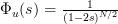
Thus the characteristic function of
is given by [3, p. 158]:
 | (7) | ||
which by using (6) is equal to:
 | |  | |
|  | (8) |
By comparing the equation (3) with (8) we see that the same characteristic function is obtained by either using the probability density function as given by (1) or by computing the characteristic function using the squared sum of
gaussian distributed random variables in conjunction with theorem (5). By virtue of the uniqueness theorem of Fourier transform pairs – the characteristic functions of a pdf is also a Fourier transform – we obtain the result that the probability density function of the squared sum of gaussian distributed random variables is equal to (1).
QED.
[1] Steven M. Kay: “Modern Spectral Estimation – Theory and Applications”, Prentice Hall, ISBN: 0-13-598582-X.
[2] Fahrmeir and Künstler and Pigeot and Tutz: “Statistik”, Springer.
[3] Papoulis, Athanasios: “Probability, Random Variables, and Stochastic Processes”, McGraw-Hill.
[4] Bronstein and Semdjajew and Musiol and Muehlig: “Taschenbuch der Mathematik”, Verlag Harri Deutsch Thun und Frankfurt am Main, ISBN: 3-8171-2003-6.
2 Responses for "Steven M. Kay: “Modern Spectral Estimation – Theory and Applications”,p. 60 exercise 3.2"
do you have the complete solution mannual of modern spectral estimation?
and may I get it?
Hi,
Morry, i am currently working towards providing a complete solution manual for Kay’s “Modern Spectral Estimation”.
I am posting the solutions of problems as soon as they are transferred into electronic format. I am planning also to provide a PDF document when all solutions are
transferred into electronic format.
Leave a reply