Lysario – by Panagiotis Chatzichrisafis
"ούτω γάρ ειδέναι το σύνθετον υπολαμβάνομεν, όταν ειδώμεν εκ τίνων και πόσων εστίν …"
Steven M. Kay: “Modern Spectral Estimation – Theory and Applications”,p. 34 exercise 2.12
Author: Panagiotis1 Apr
In [1, p. 34 exercise 2.12] we are asked to verify the equations given for the Cholesky decomposition, [1, (2.53)-(2.55)]. Furthermore it is requested to use these equations to find the inverse of the matrix given in problem [1, 2.7].
Solution: The Cholesky decomposition provides a numeric approach for solving linear equations . First the matrix
  is decomposed
as a matrix product
is decomposed
as a matrix product  , where
  is a lower triangular matrix with the elements on the main diagonal beeing ones
  , and
, and  a diagonal matrix. In order to verify [1, (2.53)] we set
  or
or
which is written analytically as:
In order to obtain the solution for the vector the previous set of equations can be rewritten as
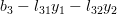
The last equations verify [1, (2.53)]. We had previously set from which we can derive
the equation  . Again expanding the previous compact matrix notation the following set of equations can be obtained:
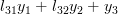
The solution for the vector can be found by rewriting the previous set of equations:
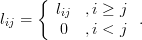
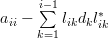
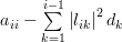
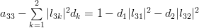
The set of equations (2,3) verify [1, (2.54)]. Equation [1, (2.55)] has still to be verified. This equation provides the algorithm to decompose the matrix. Let ![\mathbf{L}=[l_{ij}]](https://lysario.de/wp-content/cache/tex_438a67ce1c3c41c2f40f2f5c6d46ec6e.png) with
with
Thus
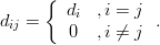
Furthermore let![\mathbf{D}=[d_{ij}]](https://lysario.de/wp-content/cache/tex_f8de7c8a00fbe8abeae4be76ac36c583.png) with
with
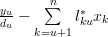
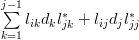
The elements of the matrix product are given by
and the elements of
of 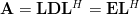 are obtained by
 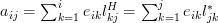 (because
  for
for  ).
When the elements
).
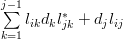
When the elements  are replaced by the corresponding sum (8) then the elements can be further expanded to:
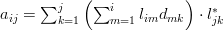 . But
. But  , for
, for  and thus:
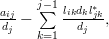
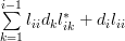
The last equation (9) is a consequence of the fact that . A recursive formula for
  can be derived when
  :
:
Equation (10) can be identified as the second part of the relation [1, (2.55)]. The first part is obtained by simply setting . In this case the second summand degenerates and the relation can be written as:
  .
From (9) by setting
.
From (9) by setting  the following relation emerges:
and again for the second summand degenerates and we obtain the relation
  .
In order to find the inverse of the real matrix given in problem [1, 2.7]:
.
In order to find the inverse of the real matrix given in problem [1, 2.7]:
we can compute the solutions by (2, 3) for which
  ,
,
 beeing the
  vector of the standard base ,
  . The inverse matrix will then be
 ![\mathbf{R}=\left[\mathbf{r}_1 \; \mathbf{r}_2 \; \mathbf{r}_3 \right]](https://lysario.de/wp-content/cache/tex_501bf87d2cc82edd44f9db5fef79ec79.png) The Cholesky decomposition of the matrix is obtained by:
The Cholesky decomposition of the matrix is obtained by:
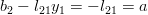
By equation (2) we obtain for :
:
and thus by (3):
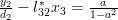
For using the formula (2):
and thus by (3):
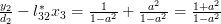
Finally for using again the formula (2):
and thus by (3):
Thus the inverse of the matrix is given by
, which is exactly the solution that was obtained in [2] for problem [1, 2.7].
[1] Steven M. Kay: “Modern Spectral Estimation – Theory and Applications”, Prentice Hall, ISBN: 0-13-598582-X.
[2] Panagiotis Chatzichrisafis: “Solution of exercise 2.7 from Kay’s Modern Spectral Estimation - Theory and Applications”, lysario.de.
Solution: The Cholesky decomposition provides a numeric approach for solving linear equations
. First the matrix is decomposed
as a matrix product , where is a lower triangular matrix with the elements on the main diagonal beeing ones , and a diagonal matrix. In order to verify [1, (2.53)] we set or
![\left[ {\begin{array}{*{20}c}
1 & 0 & \cdots & 0 \\
{l_{21} } & 1 & \cdots & 0 \\
\vdots & \vdots & \vdots & \vdots \\
{l_{n1} } & {l_{n1} } & \cdots & 1 \\
\end{array}} \right]\left[ {\begin{array}{*{20}c}
{y_1 } \\
{y_2 } \\
\vdots \\
{y_n } \\
\end{array}} \right] = \left[ {\begin{array}{*{20}c}
{b_1 } \\
{b_2 } \\
\vdots \\
{b_n } \\
\end{array}} \right]](https://lysario.de/wp-content/cache/tex_4fe2853eb9fc2bb47bc6a29b737bdb71.png) | (1) | ||
which is written analytically as:
 |  |  | |
 | |  | |
 | |  | |
 | |||
 | |  |
In order to obtain the solution for the vector
the previous set of equations can be rewritten as
| |  | |
 | |  | |
 | |  | |
| |||
 | |  | (2) |
The last equations verify [1, (2.53)]. We had previously set
from which we can derive
the equation . Again expanding the previous compact matrix notation the following set of equations can be obtained:
 | |  | |
 | |  | |
| |||
 | |  | (3) |
The solution for the vector
can be found by rewriting the previous set of equations:
 | |  | |
 | |  | |
| |||
 | |  | (4) |
| |  |
The set of equations (2,3) verify [1, (2.54)]. Equation [1, (2.55)] has still to be verified. This equation provides the algorithm to decompose the matrix
. Let with
 | (5) | ||
Thus
![\mathbf{L}^H=[l^H_{ij}]=[l^{*}_{ji}]= \left\{ {\begin{array}{*{20}c}
{l^{*}_{ji} } & {,j \ge i} \\
0 & {,i < j} \\
\end{array}} \right. .](https://lysario.de/wp-content/cache/tex_a12325a2a429c1a0cb9d1753bccdb1ef.png) | (6) | ||
Furthermore let
with
 | (7) | ||
The elements of the matrix product
are given by
| |  | (8) |
and the elements
of are obtained by (because for ).
When the elements are replaced by the corresponding sum (8) then the elements can be further expanded to:
. But , for and thus:
| |  | |
| |  | |
| |  | (9) |
The last equation (9) is a consequence of the fact that
. A recursive formula for can be derived when :
| |  | (10) |
Equation (10) can be identified as the second part of the relation [1, (2.55)]. The first part is obtained by simply setting
. In this case the second summand degenerates and the relation can be written as: .
From (9) by setting the following relation emerges:
 | |  | |
 | |  | |
| |  | (11) |
and again for
the second summand degenerates and we obtain the relation .
In order to find the inverse of the real matrix given in problem [1, 2.7]:
| | ![\left[ {\begin{array}{*{20}c}
1 & { - a} & {a^2 } \\
{ - a} & 1 & { - a} \\
{a^2 } & { - a} & 1 \\
\end{array}} \right]](https://lysario.de/wp-content/cache/tex_5e04232c7a888c06e2fd06c771ae1630.png) | (12) |
we can compute the solutions
by (2, 3) for which ,
beeing the vector of the standard base , . The inverse matrix will then be
The Cholesky decomposition of the matrix is obtained by:
 | |  | |
 | |  | |
 | |  | |
 | |  | |
 | | 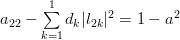 | |
 | |  | |
 | |  | |
|  |
By equation (2) we obtain for
:
| |  | |
| |  | |
| |  | |
and thus by (3):
 | |  | |
 | |  | |
 | |  |
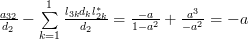
For
using the formula (2):
| |  | |
| |  | |
| |  | |
and thus by (3):
 | |  | |
 | |  | |
 | |  |
Finally for
using again the formula (2):
| | | |
| |  | |
| |  | |
and thus by (3):
 | |  | |
 | | | |
 | |  |
Thus the inverse of the matrix
is given by
 | | ![\left[ {\begin{array}{*{20}c}
\frac{1}{1-a^2} & {\frac{a}{1-a^2}} & {0 } \\
{\frac{a}{1-a^2}} & \frac{1+a^2}{1-a^2} & {\frac{a}{1-a^2}} \\
{0 } & {\frac{a}{1-a^2}} & \frac{1}{1-a^2} \\
\end{array}} \right]](https://lysario.de/wp-content/cache/tex_9ba0fb20a31488145591508dfedfc986.png) | (13) |
| ![\frac{1}{(1-a^2)^2}\left[ {\begin{array}{*{20}c}
1-a^2 & a-a^3 & 0 \\
a-a^3 & 1-a^4 & a-a^3 \\
0 & a-a^3 & 1-a^2 \\
\end{array}} \right]](https://lysario.de/wp-content/cache/tex_5445fcda9b3586ed6b29283a37e53eb7.png) | (14) |
, which is exactly the solution that was obtained in [2] for problem [1, 2.7].
[1] Steven M. Kay: “Modern Spectral Estimation – Theory and Applications”, Prentice Hall, ISBN: 0-13-598582-X.
[2] Panagiotis Chatzichrisafis: “Solution of exercise 2.7 from Kay’s Modern Spectral Estimation - Theory and Applications”, lysario.de.
One Response for "Steven M. Kay: “Modern Spectral Estimation – Theory and Applications”,p. 34 exercise 2.12"
[...] matrix , assuming are the elements of the matrix , are given by [1, p.30, (2.55)] (see also [3, relations (10) and (11) ]): and the elements of the matrix are given by the relation: The corresponding [...]
Leave a reply