Lysario – by Panagiotis Chatzichrisafis
"ούτω γάρ ειδέναι το σύνθετον υπολαμβάνομεν, όταν ειδώμεν εκ τίνων και πόσων εστίν …"
Steven M. Kay: “Modern Spectral Estimation – Theory and Applications”,p. 62 exercise 3.18
Author: Panagiotis24 Aug
In [1, p. 62 exercise 3.18] we are asked to find the temporal autocorrelation function for the real sinusoidal random process of Problem [1, p. 62 exercise 3.16]:
as . As a second step we are asked to determine if the random process autocorrelation ergodic.
Solution: The sinusoidal process of Problem [1, p. 62 exercise 3.16] is given by![x[n]=A \cos(2\pi f_{0}n+\phi)](https://lysario.de/wp-content/cache/tex_c2f33921dab216dfd22261344f21fadd.png) , and the autocorrelation function was found to be equal to (see solution of exercise 3.16 [2])
, and the autocorrelation function was found to be equal to (see solution of exercise 3.16 [2]) ![r_{xx}[k]=\frac{A^{2}}{2} \cos(2\pi f_{0}k)](https://lysario.de/wp-content/cache/tex_9f26223331739c3c8412b538256a496f.png) . The temporal autocorrelation is equal to :
. The temporal autocorrelation is equal to :
The previous relation can be furthermore simplified by the property of trigonometric functions [3, p. 810] :
and thus the autocorrelation can be written as:
Again it is possible to further simplify the previous relation, this time by using the following trigonometric formula [3, p. 810]:
Because the sinus function is odd the symmetric sum
  equals zero. Generally the same is not true for the cosine sum. For
  for example the sum
  equals
  and thus even for the temporal autocorrelation function will be in error to the true autocorrelation function.
In general it is true that
and thus even for the temporal autocorrelation function will be in error to the true autocorrelation function.
In general it is true that  .
The error to the true autocorrelation function is equal to
.
The error to the true autocorrelation function is equal to  , and thus the process is in general not autocorrelation ergodic, because as we have shown for e.g. the temporal autocorrelation doesn’t even converge for large
  . That is:
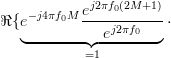
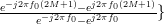
While it is true that there are frequencies for which the temporal autocorrelation doesn’t converge, there are also cases when the process is autocorrelation ergodic. To see this we have to further simplify the relation for the temporal autocorrelation. The sum
  can be further simplified, by using
  ,
and observing that the resulting sum is a geometric progression ([3, p. 7]
,
and observing that the resulting sum is a geometric progression ([3, p. 7]  ) with
  :
:
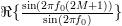
Using this identity the error to the true autocorrelation function can be rewritten as:
Thus by only imposing that the process is autocorrelation ergodic.
[1] Steven M. Kay: “Modern Spectral Estimation – Theory and Applications”, Prentice Hall, ISBN: 0-13-598582-X.
[2] Chatzichrisafis: “Solution of exercise 3.16 from Kay’s Modern Spectral Estimation - Theory and Applications.”.
[3] Granino A. Korn and Theresa M. Korn: “Mathematical Handbook for Scientists and Engineers”, Dover, ISBN: 978-0-486-41147-7.
![\hat{r}_{xx}[k]=\frac{1}{2M+1}\sum\limits_{n=-M}^{M}x[n]x[n+k]](https://lysario.de/wp-content/cache/tex_e2a95ef4fe5209acc420201c8b3143bb.png) | |||
as
. As a second step we are asked to determine if the random process autocorrelation ergodic.
Solution: The sinusoidal process of Problem [1, p. 62 exercise 3.16] is given by
, and the autocorrelation function was found to be equal to (see solution of exercise 3.16 [2]) . The temporal autocorrelation is equal to :
![\hat{r}_{xx}[k]](https://lysario.de/wp-content/cache/tex_ca6151c7d846302aeb171d16bcaf24ce.png) |  |  |
The previous relation can be furthermore simplified by the property of trigonometric functions [3, p. 810] :
 | (1) | ||
and thus the autocorrelation can be written as:
| |  | |
|  | ||
 |  | ||
|  | ||
|  | ||
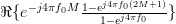
Again it is possible to further simplify the previous relation, this time by using the following trigonometric formula [3, p. 810]:
 | (2) | ||
| | | |
| 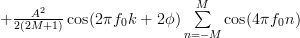 | ||
| 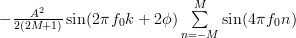 | ||
Because the sinus function is odd
the symmetric sum equals zero. Generally the same is not true for the cosine sum. For for example the sum equals and thus even for the temporal autocorrelation function will be in error to the true autocorrelation function.
In general it is true that .
The error to the true autocorrelation function is equal to , and thus the process is in general not autocorrelation ergodic, because as we have shown for e.g. the temporal autocorrelation doesn’t even converge for large . That is:
| | | |
| | ||
| ![r_{xx}[k]+\epsilon.](https://lysario.de/wp-content/cache/tex_b0dd2042185ab85bec7332dff3ee8e01.png) |
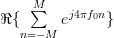
While it is true that there are frequencies
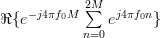
for which the temporal autocorrelation doesn’t converge, there are also cases when the process is autocorrelation ergodic. To see this we have to further simplify the relation for the temporal autocorrelation. The sum can be further simplified, by using ,
and observing that the resulting sum is a geometric progression ([3, p. 7] ) with :
 | |  | |
|  | ||
|  | ||
|  | ||
|  | ||
|  | ||
|  |
Using this identity the error to the true autocorrelation function can be rewritten as:
 | |  | |
 |  |  | |
 | |  |
Thus by only imposing that
the process is autocorrelation ergodic.[1] Steven M. Kay: “Modern Spectral Estimation – Theory and Applications”, Prentice Hall, ISBN: 0-13-598582-X.
[2] Chatzichrisafis: “Solution of exercise 3.16 from Kay’s Modern Spectral Estimation - Theory and Applications.”.
[3] Granino A. Korn and Theresa M. Korn: “Mathematical Handbook for Scientists and Engineers”, Dover, ISBN: 978-0-486-41147-7.
Leave a reply