Lysario – by Panagiotis Chatzichrisafis
"ούτω γάρ ειδέναι το σύνθετον υπολαμβάνομεν, όταν ειδώμεν εκ τίνων και πόσων εστίν …"
Steven M. Kay: “Modern Spectral Estimation – Theory and Applications”,p. 61 exercise 3.8
Author: Panagiotis22 Sep
In [1, p. 61 exercise 3.8] we are asked to prove that the sample mean is a sufficient statistic for the mean under the conditions of [1, p. 61 exercise 3.4].
Assuming that  is known. We are asked to find the MLE of the mean by maximizing
  .
.
Solution: By definition [1, p. 48] a sufficient statistic of
of  if the conditional probability density function
  does not depend on . By the Neyman-Fisher factorization theorem the statistic will be sufficient if and only if it is possible to write the PDF as:
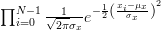
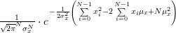
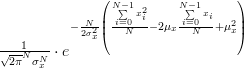
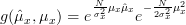
The joint p.d.f is given by:
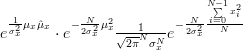
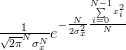
Setting
and
we see at once that the equation (2) has the form of the Neyman-Fisher factorization theorem (1), thus is sufficient.
The MLE of for the measurement
is sufficient.
The MLE of for the measurement  is obtained by:
Thus the MLE estimator of is equal to the sample mean as already obtained in [2]. QED.
[1] Steven M. Kay: “Modern Spectral Estimation – Theory and Applications”, Prentice Hall, ISBN: 0-13-598582-X.
[2] Chatzichrisafis: “Solution of exercise 3.7 from Kay’s Modern Spectral Estimation - Theory and Applications”.
is known. We are asked to find the MLE of the mean by maximizing .
Solution: By definition [1, p. 48] a sufficient statistic
of if the conditional probability density function does not depend on . By the Neyman-Fisher factorization theorem the statistic will be sufficient if and only if it is possible to write the PDF as:
 | (1) | ||
The joint p.d.f is given by:
 |  |  | |
|  | ||
|  | ||
|  | (2) |
Setting
 | |||
and
 | |  | |
| 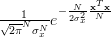 |
we see at once that the equation (2) has the form of the Neyman-Fisher factorization theorem (1), thus
is sufficient.
The MLE of for the measurement is obtained by:
 | |  | |
 | | | |
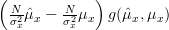 | |  | (3) |
| |  | (4) |
Thus the MLE estimator of
is equal to the sample mean as already obtained in [2]. QED.[1] Steven M. Kay: “Modern Spectral Estimation – Theory and Applications”, Prentice Hall, ISBN: 0-13-598582-X.
[2] Chatzichrisafis: “Solution of exercise 3.7 from Kay’s Modern Spectral Estimation - Theory and Applications”.
Leave a reply