Lysario – by Panagiotis Chatzichrisafis
"ούτω γάρ ειδέναι το σύνθετον υπολαμβάνομεν, όταν ειδώμεν εκ τίνων και πόσων εστίν …"
Steven M. Kay: “Modern Spectral Estimation – Theory and Applications”,p. 61 exercise 3.11
Author: Panagiotis29 Jan
In [1, p. 61 exercise 3.11] it is asked to repeat problem [1, p. 61 exercise 3.10] (see also the solution [2] ) for the general case when the predictor is given as
Furthermore we are asked to show that the optimal prediction coefficients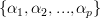 are found by solving [1, p. 157, eq. 6.4 ] and the minimum prediction error power is given by [1, p. 157, eq. 6.5 ].
Solution: The equation for determining the optimal prediction coefficients from [1, p. 157, eq. 6.4 ] is given by:
whereas the minimum MSE is given by [1, p. 157, eq. 6.5 ] as:
Using the orthogonality principle we have to obtain the coefficients that are making the observed data
 ![x_[n-k] \; ,k=1,...,p](https://lysario.de/wp-content/cache/tex_138eb6ffdc0e7272e6f59fef3948a31c.png) orthogonal to the error
orthogonal to the error ![\hat{x}[n]-x[n]](https://lysario.de/wp-content/cache/tex_0e943b2a836cdeeef26e3e0e6cf98fda.png) that is:
that is:
We see that this is the form of (2), thus the first part of the exercise is solved. The previous relation is a linear equation in the variables , and setting
![\mathbf{r}_{xx}=\left[\begin{array}{cccc}r_{xx}[1] & r_{xx}[2] & ... & r_{xx}[p]\end{array}\right]^{T}](https://lysario.de/wp-content/cache/tex_49651c1a787eb79c1744c1dab34b0b80.png) ,
, ![\mathbf{\alpha}=\left[\begin{array}{cccc}\alpha_{1} & \alpha_{1}& ... & \alpha_{p} \end{array}\right]^{T}](https://lysario.de/wp-content/cache/tex_2ccaa04b690c2bc70bf93fcdf18d935b.png) and
and
the linear equations can be written in matrix notation as:
The previous relation provides the solution for the optimum prediction parameters. The MSE for those parameters is
Let![\mathbf{x}=\left[\begin{array}{ccc} x[n-1] & \cdots & x[n-p] \end{array}\right]^{T}](https://lysario.de/wp-content/cache/tex_a0cdf117e1c185c306fc3a3fa46dd720.png) then because
then because 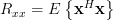 equation (7) can be written as:
Because the mean squared error can be reduced to:
We note that the last formula was obtained by replacing ,
, ![r^{\ast}_{xx}[k]=r_{xx}[-k]](https://lysario.de/wp-content/cache/tex_6a9fc40b5c629caa1ac98343de3a37d0.png) and writing out the resulting inner product. The last equation is the same as the one given at (3) in [1, p. 157, eq. 6.5 ]. Using the orthogonality principle the result can be found even faster because:
and writing out the resulting inner product. The last equation is the same as the one given at (3) in [1, p. 157, eq. 6.5 ]. Using the orthogonality principle the result can be found even faster because:
Applying the orthogonality principle to the last term of the previous equation we obtain![E\left\{x^{\ast}[n-l]\left( x[n]+\sum_{k=1}^{p}\alpha_{k}x[n-k] \right)\right\} =0](https://lysario.de/wp-content/cache/tex_1baa3a56d3f0f1b89cf97cb291ec3061.png) , and thus the MSE is equal to:
, and thus the MSE is equal to:
The previous equation is again the same as the one given at (3) in [1, p. 157, eq. 6.5 ]. We have thus proven using the orthogonality principle [1, p. 157, eq. 6.4 ] and [1, p. 157, eq. 6.5 ]. QED.
[1] Steven M. Kay: “Modern Spectral Estimation – Theory and Applications”, Prentice Hall, ISBN: 0-13-598582-X.
[2] Chatzichrisafis: “Solution of exercise 3.10 from Kay’s Modern Spectral Estimation - Theory and Applications”.
![\hat{x}[n]=-\sum\limits_{k=1}^{p}\alpha_{k}x[n-k].](https://lysario.de/wp-content/cache/tex_e9899bf3e42bcb01eecd9ca3794e97db.png) | (1) | ||
Furthermore we are asked to show that the optimal prediction coefficients
are found by solving [1, p. 157, eq. 6.4 ] and the minimum prediction error power is given by [1, p. 157, eq. 6.5 ].
Solution: The equation for determining the optimal prediction coefficients from [1, p. 157, eq. 6.4 ] is given by:
![r_{xx}[k]=-\sum\limits_{l=1}^{p}\alpha_{l}r_{xx}[k-l] \;,k=1,2,...,p](https://lysario.de/wp-content/cache/tex_77fd0886edab04f08c09525c4d4ed429.png) | (2) | ||
whereas the minimum MSE is given by [1, p. 157, eq. 6.5 ] as:
![\rho_{MIN}=r_{xx}[0]+\sum\limits_{k=1}^{p}\alpha_{k}r_{xx}[-k] \;, k=1,2,...,p](https://lysario.de/wp-content/cache/tex_3a9006a892d390098e5a12796afd4d62.png) | (3) | ||
Using the orthogonality principle we have to obtain the coefficients
that are making the observed data orthogonal to the error that is:
![E\{x[n-k]^{\ast} (- \hat{x}[n]+x[n]) \}](https://lysario.de/wp-content/cache/tex_6b0b284df9a28b9c8e72f6333904de6e.png) |  |  | |
![E\{ x[n-k]^{\ast} (\sum\limits_{l=1}^{p}\alpha_{k}x[n-l]+x[n])\}](https://lysario.de/wp-content/cache/tex_58d1f3eec30760a03198b1413d6bd377.png) | |  | |
![\sum\limits_{l=1}^{p}\alpha_{l}E\{ x^{\ast}[n-k]x[n-l]\}+E\{ x^{\ast}[n-k]x[n])\}](https://lysario.de/wp-content/cache/tex_c477d70dc416693dc38c37537627bf31.png) | |  | |
![\sum\limits_{l=1}^{p}\alpha_{l} r_{xx}[k-l]+r_{xx}[k]](https://lysario.de/wp-content/cache/tex_cf9f0857af6b61cab2111dcda9dc5b9c.png) | | | (4) |
We see that this is the form of (2), thus the first part of the exercise is solved. The previous relation is a linear equation in the variables
, and setting
, and
![R_{xx}=\left[\begin{array}{cccc}r_{xx}[0] & r_{xx}[-1]& \cdots&r_{xx}[-(p-1)] \\r_{xx}[1] &r_{xx}[0] &\cdots&r_{xx}[-(p-2)] \\ \vdots &\vdots & \ddots& \vdots \\ r_{xx}[p-1]&r_{xx}[p-2]&... &r_{xx}[0]\end{array}\right]](https://lysario.de/wp-content/cache/tex_325b4a4285535beb535c4d9bc12af9a9.png) | (5) | ||
the linear equations can be written in matrix notation as:
 | |  | |
 | |  | (6) |
The previous relation provides the solution for the optimum prediction parameters. The MSE for those parameters is
 | | ![E\left\{(x[n]+\sum\limits_{k=1}^{p}\alpha_{k}x[n-k])^{\ast}(x[n]+\sum\limits_{k=1}^{p}\alpha_{k}x[n-k])\right\}](https://lysario.de/wp-content/cache/tex_c73490f81066f408f9cbf882df9fa051.png) | |
| ![E\left\{ x[n]^{\ast}x[n]\right\}+ \sum\limits_{k=1}^{p}\alpha_{k}E\left\{x^{\ast}[n]x[n-k]\right\}](https://lysario.de/wp-content/cache/tex_fce5f22e0f0a1a7a498e46ccb34ae092.png) | ||
 | ![+ \sum\limits_{k=1}^{p}\alpha^{\ast}_{k}E\left\{x[n]x^{\ast}[n-k]\right\}](https://lysario.de/wp-content/cache/tex_ffb2217f7b04043c59c207b823b8f617.png) | ||
| ![+ E\left\{ \left(\sum\limits_{k=1}^{p}\alpha^{\ast}_{k}x^{\ast}[n-k]\right)\left(\sum\limits_{k=1}^{p}\alpha_{k}x[n-k]\right)\right\}](https://lysario.de/wp-content/cache/tex_abcb6f7585ca47a3191f538fc2829bb1.png) | (7) |
Let
then because equation (7) can be written as:
| | | |
| | ||
| 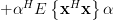 | ||
| ![r_{xx}[0]+ \sum\limits_{k=1}^{p}\alpha_{k}r_{xx}[-k]+ \sum\limits_{k=1}^{p}\alpha^{\ast}_{k}r_{xx}[k] + \mathbf{\alpha}^{H} R_{xx}\mathbf{\alpha}](https://lysario.de/wp-content/cache/tex_0aca7999c47c18ec53ed7e0aea83ef07.png) | ||
| ![r_{xx}[0]+ \mathbf{r}_{xx}^{H}\mathbf{\alpha}+ \mathbf{\alpha}^{H} \mathbf{r}_{xx} + \mathbf{\alpha}^{H} R_{xx}\mathbf{\alpha}](https://lysario.de/wp-content/cache/tex_c3ce8a944f543117026cc6a1f9c1e71d.png) |
Because
the mean squared error can be reduced to:
| | ![r_{xx}[0]- \mathbf{r}_{xx}^{H}\mathbf{R}^{-1}_{xx}\mathbf{r}_{xx}- \left(\mathbf{R}^{-1}_{xx}\mathbf{r}_{xx}\right)^{H} \mathbf{r}_{xx}](https://lysario.de/wp-content/cache/tex_0ba051c27ca40ffb1dd881d378f83cc1.png) | |
| 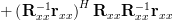 | ||
| ![r_{xx}[0]- \mathbf{r}_{xx}^{H}\mathbf{R}^{-1}_{xx}\mathbf{r}_{xx}-\mathbf{r}_{xx}^{H} \left(\mathbf{R}^{-1}_{xx}\right)^{H}\mathbf{r}_{xx} + \mathbf{r}_{xx}^{H} \left(\mathbf{R}^{-1}_{xx}\right)^{H}\mathbf{r}_{xx}](https://lysario.de/wp-content/cache/tex_3f01fcd0d85cf1b86b1b534887414ec4.png) | ||
| ![r_{xx}[0]- \mathbf{r}_{xx}^{H}\mathbf{R}^{-1}_{xx}\mathbf{r}_{xx}](https://lysario.de/wp-content/cache/tex_0f9c6d445170e978c0b9b7db9f9c1095.png) | ||
| ![r_{xx}[0]+\sum\limits_{k=1}^{p}\alpha_{k}r_{xx}[-k]](https://lysario.de/wp-content/cache/tex_64897784a2d3b4f4b09f07502638970f.png) |
We note that the last formula was obtained by replacing
, and writing out the resulting inner product. The last equation is the same as the one given at (3) in [1, p. 157, eq. 6.5 ]. Using the orthogonality principle the result can be found even faster because:
| | | |
| ![E\left\{x^{\ast}[n]\left( x[n]+\sum\limits_{k=1}^{p}\alpha_{k}x[n-k] \right)\right\}](https://lysario.de/wp-content/cache/tex_37873c7d14d0287942a533507a18adeb.png) | ||
| ![+\sum\limits_{l=1}^{p}\alpha_{l}E\left\{x^{\ast}[n-l]\left( x[n]+\sum\limits_{k=1}^{p}\alpha_{k}x[n-k] \right)\right\}](https://lysario.de/wp-content/cache/tex_3c67c4a8c7942329aa8dac35c2bdbc9e.png) |
Applying the orthogonality principle to the last term of the previous equation we obtain
, and thus the MSE is equal to:
| | | |
| ![r_{xx}[0]+\sum\limits_{k=1}^{p}\alpha_{k}r_{xx}[-k]](https://lysario.de/wp-content/cache/tex_bd3d286d10f79d06e6461179a4a49bce.png) |
The previous equation is again the same as the one given at (3) in [1, p. 157, eq. 6.5 ]. We have thus proven using the orthogonality principle [1, p. 157, eq. 6.4 ] and [1, p. 157, eq. 6.5 ]. QED.
[1] Steven M. Kay: “Modern Spectral Estimation – Theory and Applications”, Prentice Hall, ISBN: 0-13-598582-X.
[2] Chatzichrisafis: “Solution of exercise 3.10 from Kay’s Modern Spectral Estimation - Theory and Applications”.
Leave a reply